
Monitoring water quality in active mining regions is critical for environmental compliance and ESG reporting. However, analysts often struggle with complex hydrogeochemical datasets containing dozens of overlapping variables. How can we turn this overwhelming data into clear, actionable insights?
This case study demonstrates an end-to-end data science workflow to map water contamination in an anonymized industrial site (Mining Area X).
- Dimensionality Reduction: Applying Principal Component Analysis (PCA) in R to condense complex chemical variables (e.g., Sodium, Chloride, Sulfate) into a single, unified “Pollution Index.”
- Spatial Interpolation: Utilizing QGIS to predict and model contamination levels across the entire region, even in areas without direct water samples.
- Risk Identification: Creating an intuitive, data-driven heatmap that highlights the proximity of high-risk salinity zones to critical natural waterways.
By integrating unsupervised machine learning with geostatistical mapping, this project bridges the gap between raw data and spatial intelligence.
The Challenge: High-Dimensional Environmental Data
Environmental datasets are notoriously messy. The raw data for Mining Area X consisted of 74 water samples, with each sample measured across various geochemical parameters (e.g., pH, Electrical Conductivity, Alkalinity, and major ions like Na+, Cl–, and SO2-4).
Analyzing each parameter individually is time-consuming and often fails to reveal the broader spatial patterns of contamination. Furthermore, environmental variables are often highly correlated—for instance, high Sodium is almost always accompanied by high Chloride. Treating them as independent variables would be statistically redundant.
Data Pre-processing in R
Before applying any machine learning algorithm, robust data preparation is mandatory. The pre-processing workflow included:
Handling Missing Values: Removing or imputing missing records to ensure statistical validity.
Outlier Management: Identifying extreme values (which are common in pollution data) using visualization and adjusting them logarithmically where necessary to prevent them from skewing the model.
Standardization: Scaling the variables so that parameters measured in large units (like Conductivity) do not dominate parameters measured in small units (like pH).
Dimensionality Reduction: The Power of PCA
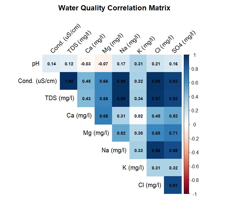
As visualized in the correlation matrix above, strong positive correlations exist between variables such as Conductivity, TDS, Sodium (Na), and Chloride (Cl). In a traditional analysis, evaluating these individually would lead to redundant conclusions.
To solve this, I applied Principal Component Analysis (PCA) using R. PCA is an unsupervised machine learning technique that identifies the underlying patterns in a dataset and compresses highly correlated variables into a smaller set of uncorrelated “Principal Components” (PCs) without losing significant information.
Visualizing the Principal Components (Biplot)
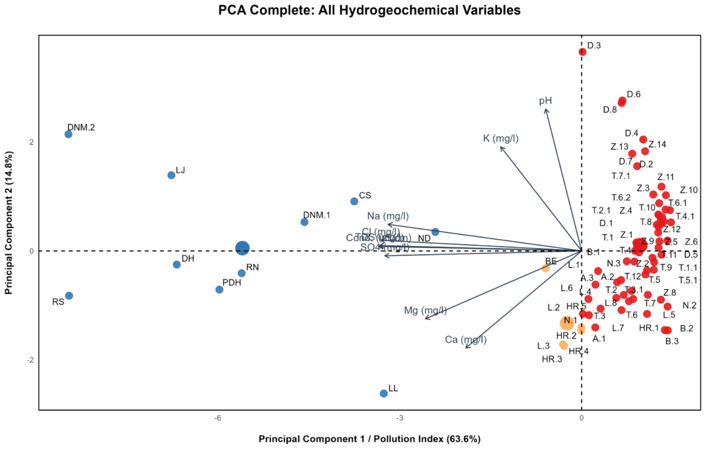
The resulting PCA biplot above reveals the hidden structure of the dataset. The arrows represent the original geochemical variables. Notably, variables associated with salinity and mineralization (Na, Cl, TDS, Conductivity) strongly drive the variance along the first Principal Component (PC1).
Therefore, instead of tracking multiple distinct chemical measurements, we can confidently use the PC1 score of each water sample as a singular, comprehensive “Pollution Index.” A higher PC1 score strongly indicates elevated salinity and contamination levels.
Deconstructing the Contamination: A Two-Pronged PCA Approach
While the initial PCA successfully condensed all variables into a single index, a closer look at the correlation matrix revealed two distinct clusters of geochemical behavior. To prevent the dominant salinity signals from overshadowing subtle natural variations, I split the data and ran two independent PCA models:
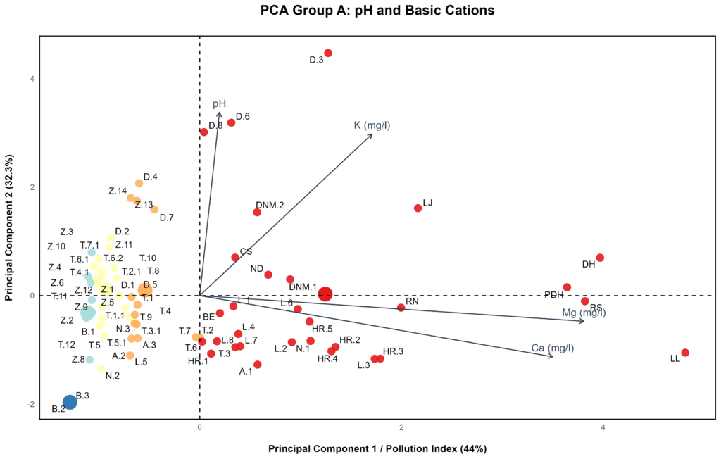
1. Group A: Natural Baseline Indicators (pH, Ca, Mg, K) The first model focuses on variables typically associated with natural rock-water interactions and baseline hydrochemistry.
- The Finding: The resulting biplot for Group A shows a wider, more scattered distribution of water samples. This indicates that natural mineralization across Mining Area X is highly variable and depends strongly on local geological conditions rather than a single point of industrial impact.
- Key Insight: Samples that score high on PC1 in this group (moving to the right of the graph) are generally rich in natural earth alkaline metals (Magnesium and Calcium), likely reflecting the dissolution of local bedrock.
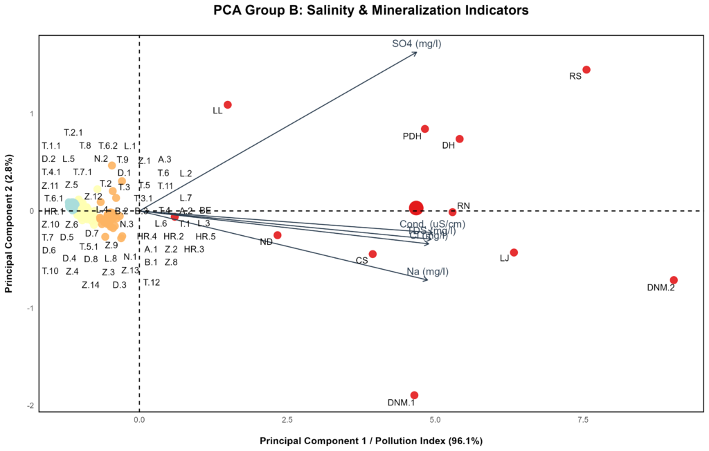
2. Group B: Salinity & Industrial Impact Indicators (Cond, TDS, Na, Cl, SO4) The second model isolates variables strongly correlated with mining effluent and surface contamination.
- Key Insight: This extreme correlation confirms that these specific chemicals are moving together as a unified “contamination plume.” The samples plotted far to the right (colored deep red) are not just naturally mineralized; they are heavily impacted by industrial salinity.
- The Finding: The biplot for Group B reveals a very different story. The arrows for Sodium (Na), Chloride (Cl), Sulfate (SO4), and Total Dissolved Solids (TDS) all pull strongly in the exact same direction (driving over 96% of the variance on PC1).
Spatial Intelligence: Bringing Data to the Map
Statistical biplots reveal the underlying relationships between chemical variables and individual samples, but they lack spatial context. To translate these abstract chemical signatures into actionable environmental intelligence, we must move from the scatter plot to the geographic map.
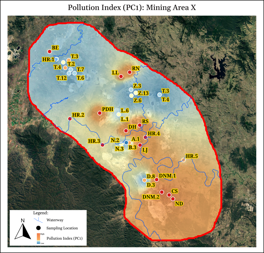
To achieve this, I utilized the Principal Component 1 (PC1) scores derived from the comprehensive PCA model (incorporating all hydrogeochemical variables). Because variables associated with industrial mineralization (Cond, TDS, Na, Cl, SO4) overwhelmingly dominate the variance along PC1, these scores serve as an exceptionally robust, singular “Pollution Index.”
By importing these PC1 scores into QGIS and applying geostatistical interpolation techniques, we can visualize the exact spatial footprint of the contamination plume across Mining Area X.
Geostatistical Insights